To obtain accurate measurements, in the physical lab environment, the camera exposure time can be adjusted through the exposureTime variable.
What is Exposure Time?
Exposure time determines how long the camera integrates incoming light.
The measured signal is proportional to the light intensity integrated over the exposure duration.
The cameras installed in the Physical Lab support exposure times in the range:
16 microseconds ≤ exposureTime ≤ 1300 microseconds.
This range allows flexibility to adapt measurements to different problem instances and optical conditions.
How Coupling Affects Intensity?
The required exposure time depends on the signal intensity, which is directly determined by the structure of the coupling matrix.
For example, a diagonal coupling matrix typically yields maximum lasing efficiency, so a shorter exposure time is sufficient. In contrast, a fully connected coupling matrix generally reduces lasing efficiency and therefore requires a longer exposure time to obtain a well-resolved signal.
As a rule of thumb
• Fewer couplings: Higher optical efficiency → stronger signal → lower exposure time is recommended.
• More couplings: Lower efficiency → weaker signal → higher exposure time is recommended.
System conditions and environmental variations may also influence intensity, exposure time is adjusted per system.
Failure Modes
1. Saturation (Exposure Too High)
The camera signal ranges from 0 to 255 (8-bit grayscale per pixel).
If the optical intensity exceeds the maximum measurable value, the recorded pixel value is clipped at 255. When many pixels reach this limit, the image appears saturated, and information about relative intensities is lost. Fringe structure becomes distorted with contrast artificially reduced, and phase extraction may become unreliable.
Symptom: Large areas with flat intensity (at 255 grayscale ).
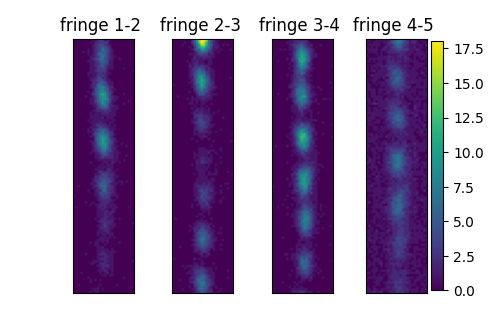
2. Underexposure (Exposure Too Low)
If the optical intensity is weak the signal to noise ratio (SNR) is decreased, contrast becomes difficult to detect.
When signal is low – SNR < 1.5 or contrast < 1, phase and contrast are set to return NaN if to avoid misleading results.
Symptom: grey level of fringes is comparable with grey level of the background.
Recommended Workflow
- 1. Start with the system default exposure time.
- 2. Inspect the returned camera image.
- 3. If saturation appears → decrease exposure.
- 4. If fringes are dim and SNR is low → increase exposure gradually, but avoid saturation.
- 5. Aim for strong, clear fringe contrast without saturation.
Once the exposure is properly set, the derived parameters (phase, contrast, energy, and SNR) will accurately reflect the laser states.
Example Workflow
1. Create a coupling matrix
import numpy
from laser_mind_client import LaserMind

size = 5
coupling_matrix = 0.5 * numpy.eye(size, dtype=numpy.complex64)
coupling = (1-0.5)/2
for i in range(size - 1):
    coupling_matrix[i,i+1] = coupling
    coupling_matrix[i+1,i] = coupling
2. Run with default exposure time
pathToRefreshTokenFile="C:\\path\\to\\your\\token.txt"
lsClient = LaserMind(pathToRefreshTokenFile=pathToTokenFile)

result = lsClient.solve_coupling_matrix_lpu(
    matrixData=coupling_matrix ,
    num_runs=1,
    average_over=1,
    num_neighbors=1,
    waitForSolution=True
)
print("Exposure time:", result["data"]["exposure_time"])Note: The default exposure time in this example was 100 miliseconds.
3. Observe output images
def view_solution_img(result):
solutions = result["data"]["solutions"] # list of per-run dictionaries
imgs = solutions[0]["image_problem_list"]
import matplotlib.pyplot as plt
plt.figure()
vmin = min(img.min() for img in imgs[1:size])
vmax = max(img.max() for img in imgs[1:size])
for laserIdx in range(1,size):
plt.subplot(1,size-1,laserIdx)
plt.imshow(imgs[laserIdx], vmin=vmin, vmax=vmax)
plt.title(f"fringe {laserIdx}-{laserIdx+1} ")
plt.xticks([])
plt.yticks([])
plt.colorbar()
plt.show()
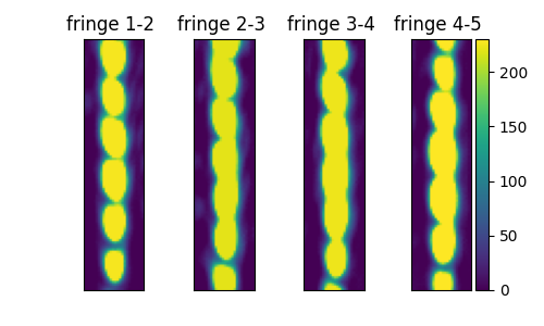
view_solution_img(result)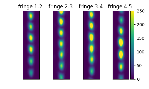
The resulting image has visible fringes with good contrast. There are saturated pixels at the fringe peaks.
4. Run with adjusted exposure time
result = lsClient.solve_coupling_matrix_lpu(
    matrixData=coupling_matrix ,
    num_runs=1,
    average_over=1,
    exposure_time=50,
    num_neighbors=1,
    waitForSolution=True
)
print("Exposure time:", result["data"]["exposure_time"])

view_solution_img(result)5. Observe again
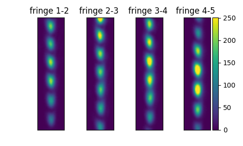
Confirm that fringe visibility has improved by checking that the maximum gray level remains below 255 (no saturation) and is clearly above the background gray level.